Optimization by Grid search

In this section, we will explain how to perform a grid-type search to analyze atomic coordinates from diffraction data. The grid type search is compatible with MPI. It is necessary to prepare the data file MeshData.txt that defines the search grid in advance.

Location of the sample files

The sample files are located in sample/mapper. The following files are stored in the folder:

• base directory

  Directory that contains reference files to proceed with calculations in the main program. The reference files include: exp.d, rfac.d, short.t, tleed.o, tleed4.i, and tleed5.i.

• input.toml

  Input file of the main program.

• MeshData.txt

  Data file for the search grid.

• ref_ColorMap.txt

  A file to check if the calculation was performed correctly (the answer to ColorMap.txt obtained by doing this tutorial).

• prepare.sh, do.sh

  Script prepared for bulk calculation of this tutorial.

Below, we will describe these files and then show the actual calculation results.

Reference files

tleed4.i, tleed5.i, and rfac.d are the parameter files for satleed. The atomic coordinates to be optimized should be replaced by the keywords such as opt000 or opt001 in tleed4.i. exp.d is the reference experimental data. short.t and tleed.o are the input data that have been generated by using satl1.exe.

The search grid is given by MeshData.txt. In this tutorial, the content of MeshData.txt is as follows:

0 -0.1   0
1 -0.05  0
2 0      0
3 0.05   0
4 0.1    0
5 -0.1   0.05
6 -0.05  0.05
7 0      0.05
8 0.05   0.05
9 0.1    0.05

The first column denotes the sequential id, and the second and subsequent columns denote the parameter values for opt000 and opt001 in tleed4.i.

Input file

This section describes the input file for the main program, input.toml. The details of input.toml can be found in the input file section of the manual. The following is the content of input.toml in the sample file.

[base]
dimension = 2
output_dir = "output"

[solver]
name = "leed"
[solver.config]
path_to_solver = "./leedsatl/satl2.exe"
[solver.reference]
path_to_base_dir = "./base"

[algorithm]
name = "mapper"
label_list = ["z1", "z2"]
[algorithm.param]
mesh_path = "./MeshData.txt"

First, [base] section is explained.

• dimension is the number of variables to be optimized. In this case, it is 2 since we are optimizing two variables as described in tleed4.i.

• output_dir is the name of directory for the outputs. If it is omitted, the results are written in the directory in which the program is executed.

[solver] section specifies the solver to be used inside the main program and its settings.

• name is the name of the solver you want to use. In this tutorial it is leed.

The solver can be configured in the subsections [solver.config] and [solver.reference].

[solver.config] section specifies options for reading the output file produced by satl2.exe that is called from the main program.

• path_to_solver is the command name of satl2.exe. It is specified as a path to the executable file, or searched from the PATH environment variable.

[solver.reference] section specifies the location of the experimental data and the range to read.

• path_to_base_dir specifies the path to the directory for the reference data.

[algorithm] section specifies the algorithm to use and its settings.

• name is the name of the algorithm you want to use. In this tutorial we will use mapper since we will be using grid-search method.

• label_list is a list of label names to be attached to the output of opt000 and opt001.

[algorithm.param] section specifies the parameters for the search algorithm.

• mesh_path is the file name of the search grid.

For details on other parameters that can be specified in the input file, please see the Input File section of the manual.

Calculation execution

First, move to the folder where the sample files are located. (We assume that you are directly under the directory where you downloaded this software.)

$ cd sample/mapper

Using setup.sh, download and compile satleed.

$ sh setup.sh

satl1.exe and satl2.exe will be created in the directory leedsatl. Then, run the main program. The computation time will take only a few seconds on a normal PC.

$ mpiexec -np 4 odatse-LEED input.toml | tee log.txt

Here, the calculation using MPI parallel with 4 processes will be done. When executed, a folder for each MPI rank will be created in output, and the results of the calculations are stored there. The standard output will be shown like as follows.

Iteration : 1/33
Read experiment.txt
mesh before: [1.0, 6.0, 6.0]
z1 =  6.00000
z2 =  6.00000
[' 6.00000', ' 6.00000']
PASS : degree in lastline = 7.0
PASS : len(calculated_list) 70 == len(convolution_I_calculated_list)70
R-factor = 0.04785241875354398
...

z1 and z2 are the candidate parameters for each mesh and R-factor is the function value at that point. Finally, the R-factor calculated at all the points on the grid will be written to ColorMap.txt. In this case, the following results will be obtained.

-0.100000 0.000000 0.319700
-0.050000 0.000000 0.212100
0.000000 0.000000 0.189500
0.050000 0.000000 0.502300
0.100000 0.000000 0.941600
-0.100000 0.050000 0.318600
-0.050000 0.050000 0.206600
0.000000 0.050000 0.190500
0.050000 0.050000 0.506200
0.100000 0.050000 0.933200
...

The first and second columns contain the values of opt000 and opt001, and the third column contains the R-factor.

Note that do.sh is available as a script for batch calculation. In do.sh, the difference between ColorMap.dat and ref_ColorMap.dat is also examined. Here is what it does, without further explanation.

#!/bin/sh

sh prepare.sh

time mpiexec -np 4 odatse-LEED input.toml

echo diff output/ColorMap.txt ref_ColorMap.txt
res=0
diff output/ColorMap.txt ref_ColorMap.txt || res=$?
if [ $res -eq 0 ]; then
  echo TEST PASS
  true
else
  echo TEST FAILED: ColorMap.txt and ref_ColorMap.txt differ
  false
fi

Visualization of calculation results

By plotting ColorMap.txt, we can estimate the region where the value of R-factor becomes small. In this case, the following command will create a two-dimensional parameter space diagram ColorMapFig.png.

$ python3 plot_colormap_2d.py

Looking at the generated figure, we can see that it has the minimum value around (-0.02, ±0.1).

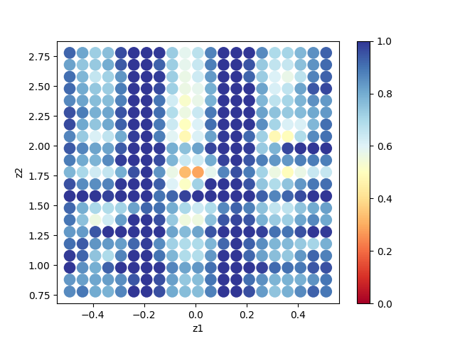
Fig. 1 R-factor on a two-dimensional parameter space.