グリッド型探索
ここでは、グリッド型探索を行い、分光スペクトルから原子座標を解析する方法について説明します。 グリッド型探索はMPIに対応しています。 探索グリッドは入力パラメータをもとに等間隔のメッシュとして生成します。
サンプルファイルの場所
サンプルファイルは sample/mapper にあります。
フォルダには以下のファイルが格納されています。
mock_data.txt,template.txtメインプログラムでの計算を進めるための参照ファイル
ref_ColorMap.txt計算が正しく実行されたか確認するためのファイル(本チュートリアルを行うことで得られる
ColorMap.txtの回答)。input.tomlメインプログラムの入力ファイル
prepare.sh,do.sh本チュートリアルを一括計算するために準備されたスクリプト
以下、これらのファイルについて説明したあと、実際の計算結果を紹介します。
参照ファイルの説明
template.txt は FEFF の入力ファイルのテンプレートです。
ここでは、S原子の座標 x, y, z のうち、計算量を減らすために z = -1.60 に固定して x, y の 2次元空間の探索を行います。
以下にファイルの内容を示しますが、 @x, @y が動かすパラメータに相当します。
リファレンスとなる測定データを模したデータは mock_data.txt です。偏光方向を3通りにとったスペクトルデータが格納されています。
* This feff.inp file generated by ATOMS, version 2.50
* ATOMS written by and copyright (c) Bruce Ravel, 1992-1999

* -- * -- * -- * -- * -- * -- * -- * -- * -- * -- * -- * -- * -- * -- *
*       total mu =      725.4 cm^-1, delta mu =      610.0 cm^-1
*       specific gravity = 12.006, cluster contains   55 atoms.
* -- * -- * -- * -- * -- * -- * -- * -- * -- * -- * -- * -- * -- * -- *
*       mcmaster corrections:  0.00020 ang^2 and  0.770E-07 ang^4
* -- * -- * -- * -- * -- * -- * -- * -- * -- * -- * -- * -- * -- * -- *

TITLE   Sample_data

EDGE      K
S02       1.0

*         pot    xsph  fms   paths genfmt ff2chi
CONTROL   1      1      1      1      1      1
PRINT     0      0      0      0      0      0

*         r_scf   [ l_scf  n_scf  ca ]
*SCF       6.05142     0     15     0.1


EXAFS    20
RPATH    6

*         kmax  [ delta_k  delta_e ]
*XANES     4.0     0.07     0.5
*         r_fms     [ l_fms ]
*FMS       6.05142    0
*
*RPATH     0.10000
*         emin  emax  resolution
*LDOS      -20    20   0.1


POTENTIALS
*   ipot   z [ label   l_scmt  l_fms  stoichiometry ]
       0   28    Ni
       1   16    S
       2    8     O
NLEG         2

*CRITERIA     4.00     2.50

*DEBYE        300.00   340.00

* CORRECTION 4.50 0.5
* RMULTIPLIER 1.00
* ION 0 0.2
* ION 1 0.2

*         ixc  [ Vr  Vi ]
EXCHANGE  0    -5    0
SIG2  0.0016
POLARIZATION   @Ex @Ey @Ez

ATOMS
0.0000 0.0000 0.0000 0 Ni
@x @y -1.6000 1 S
1.1400 1.2800 0.9700 2 O
入力ファイルの説明
ここでは、メインプログラム用の入力ファイル input.toml について説明します。
パラメータの詳細についてはマニュアルの入出力の章を参照してください。
以下は、サンプルファイルにある input.toml の内容です。
[base]
dimension = 2
output_dir = "output"

[solver]
name = "feff"

[solver.config]
feff_exec_file  = "feff85L"
feff_output_file = "chi.dat"
#remove_work_dir = true
#use_tmpdir = true

[solver.param]
string_list = ["@x", "@y"]
polarization_list = ["@Ex", "@Ey", "@Ez"]
polarization = [ [0,1,0], [1,0,0], [0,0,1] ]
calculated_first_k = 3.6
calculated_last_k = 10

[solver.reference]
path_epsilon = "mock_data.txt"

[algorithm]
name = "mapper"
label_list = ["x_S", "y_S"]

[algorithm.param]
min_list = [-2.0, -2.0]
max_list = [ 2.0,  2.0]
num_list = [21, 21]
最初に [base] セクションについて説明します。
dimensionは最適化したい変数の個数で、今の場合はtemplate.txtで説明したように2つの変数の最適化を行うので、2を指定します。output_dirは出力先のディレクトリ名です。省略した場合はプログラムを実行したディレクトリになります。
[solver] セクションではメインプログラムの内部で使用するソルバーとその設定を指定します。
nameは使用したいソルバーの名前です。feffに固定されています。
ソルバーの設定は、サブセクションの [solver.config], [solver.param], [solver.reference] で行います。
[solver.config] セクションではメインプログラム内部で呼び出す feff85L に関するオプションを指定します。
feff_exec_fileは FEFF の実行ファイルのパスを指定します。feff_output_fileは FEFF の出力ファイルのうち、XAFS スペクトルデータを格納するファイルを指定します。remove_work_dirは各 iteration ごとに FEFF の出力ファイルを削除するオプションです。use_tmpdirは FEFF の出力ファイルの書き出し先を /tmp にするオプションです。
[solver.param] セクションでは FEFF の入力に関するオプションを指定します。
string_listは、template.txtで読み込む、動かしたい変数の名前のリストです。polarization_listは、template.txtで読み込む、偏光ベクトルの要素の名前のリストです。polarizationは、偏光ベクトルのセットを指定します。calculated_first_k,calculated_last_kは、計算結果と測定データを比較する際の波数 \(k\) の範囲(下端・上端)を指定します。
[solver.reference] セクションでは、リファレンスとなる測定データに関するオプションを指定します。
path_epsilonは実験データが置いてあるパスを指定します。
[algorithm] セクションでは、使用するアルゴリスムとその設定をします。
nameは使用したいアルゴリズムの名前です。このチュートリアルではグリッド探索による解析を行うのでmapperを指定します。label_listは、変数の値を出力する際につけるラベル名のリストです。
[algorithm.param] セクションでは、探索するパラメータの範囲や初期値を指定します。
min_list,max_list,num_listは、探索グリッドの範囲と分割数を指定します。
その他、入力ファイルで指定可能なパラメータの詳細については入出力の章をご覧ください。
計算実行
最初にサンプルファイルが置いてあるフォルダへ移動します(以下、本ソフトウェアをダウンロードしたディレクトリ直下にいることを仮定します).
$ cd sample/mapper
順問題の時と同様に feff85L をコピーします。
$ cp ../feff/feff85L .
メインプログラムを実行します。以下のコマンドではプロセス数4のMPI並列を用いた計算を行っています。(計算時間は通常のPCで数分程度で終わります。)
$ mpiexec -np 4 odatse-XAFS input.toml | tee log.txt
実行すると、output ディレクトリ内に各ランクのフォルダが作成され、その中にグリッドのidがついたサブフォルダ LogXXXX_00000000 (XXXX がグリッドのid) が作成されます。
また、以下の様な出力が標準出力に書き出されます。
name            : mapper
label_list      : ['x_S', 'y_S']
param.min_list  : [-2, -2]
param.max_list  : [2, 2]
param.num_list  : [21, 21]
Iteration : 1/441
@x = -2.00000000
@y = -2.00000000
R-factor = 19.739646449543752 Polarization [0.0, 1.0, 0.0] R-factor1 = 2.23082630928769  Polarization [1.0, 0.0, 0.0] R-factor2 = 3.745102742186708  Polarization [0.0, 0.0, 1.0] R-factor3 = 53.243010297156864
Iteration : 2/441
@x = -1.80000000
@y = -2.00000000
R-factor = 15.870615265918195 Polarization [0.0, 1.0, 0.0] R-factor1 = 2.465225144249503  Polarization [1.0, 0.0, 0.0] R-factor2 = 3.7116841611214517  Polarization [0.0, 0.0, 1.0] R-factor3 = 41.43493649238363
Iteration : 3/441
@x = -1.60000000
@y = -2.00000000
R-factor = 12.4966032440396 Polarization [0.0, 1.0, 0.0] R-factor1 = 3.4464214082242046  Polarization [1.0, 0.0, 0.0] R-factor2 = 2.6218600524063693  Polarization [0.0, 0.0, 1.0] R-factor3 = 31.421528271488228
Iteration : 4/441
@x = -1.40000000
@y = -2.00000000
R-factor = 11.698213396270965 Polarization [0.0, 1.0, 0.0] R-factor1 = 3.4791684719050933  Polarization [1.0, 0.0, 0.0] R-factor2 = 1.6240174174998872  Polarization [0.0, 0.0, 1.0] R-factor3 = 29.991454299407913
Iteration : 5/441
@x = -1.20000000
@y = -2.00000000
R-factor = 14.299726412681139 Polarization [0.0, 1.0, 0.0] R-factor1 = 2.2280314879817467  Polarization [1.0, 0.0, 0.0] R-factor2 = 1.5332463231108493  Polarization [0.0, 0.0, 1.0] R-factor3 = 39.13790142695082
Iteration : 6/441
@x = -1.00000000
@y = -2.00000000
R-factor = 21.44097816422594 Polarization [0.0, 1.0, 0.0] R-factor1 = 3.7563622860968673  Polarization [1.0, 0.0, 0.0] R-factor2 = 1.810765574876649  Polarization [0.0, 0.0, 1.0] R-factor3 = 58.7558066317043
Iteration : 7/441
@x = -0.80000000
@y = -2.00000000
R-factor = 28.455902096414444 Polarization [0.0, 1.0, 0.0] R-factor1 = 6.512305703044855  Polarization [1.0, 0.0, 0.0] R-factor2 = 2.004528093101423  Polarization [0.0, 0.0, 1.0] R-factor3 = 76.85087249309706
...
@x, @y に各メッシュでの候補パラメータと、その時の R-factor が出力されます。
最終的にグリッド上の全ての点で計算された R-factor は output/ColorMap.txt に出力されます。
今回の場合は
-2.000000 -2.000000 19.739646
-1.800000 -2.000000 15.870615
-1.600000 -2.000000 12.496603
-1.400000 -2.000000 11.698213
-1.200000 -2.000000 14.299726
-1.000000 -2.000000 21.440978
-0.800000 -2.000000 28.455902
...
のように得られます。1, 2列目に @x, @y の値が、3列目に R-factor が記載されます。
なお、一括計算するスクリプトとして do.sh を用意しています。
do.sh では ColorMap.dat と ref_ColorMap.dat の差分も比較しています。
以下、説明は割愛しますが、その中身を掲載します。
#!/bin/sh

sh prepare.sh

time mpiexec -np 4 odatse-XAFS input.toml

echo diff output/ColorMap.txt ref_ColorMap.txt
res=0
diff output/ColorMap.txt ref_ColorMap.txt || res=$?
if [ $res -eq 0 ]; then
  echo TEST PASS
  true
else
  echo TEST FAILED: ColorMap.txt and ref_ColorMap.txt differ
  false
fi
計算結果の可視化
ColorMap.txt を図示することで、 R-factor の小さいパラメータがどこにあるかを推定することができます。
以下のコマンドを入力すると 2次元パラメータ空間の図 ColorMapFig.png が作成されます。
$ python3 plot_colormap_2d.py -o ColorMapFig.png
作成された図を見ると、(\(\pm 1.2\), \(\pm 0.8\)) 付近に最小値があることがわかります。
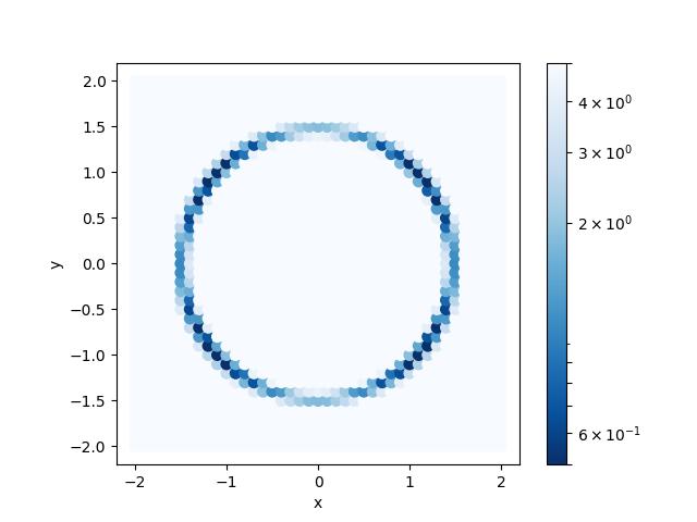
S原子の x, y 座標に対する R-factor のプロット。z = -1.60 に固定。