XAFS Solver
In this section, we will explain how to install and test FEFF.
Download and Install
First, you need to obtain the source package of odatse-XAFS from the repository.
$ git clone https://github.com/2DMAT/odatse-XAFS.git
$ cd odatse-XAFS
Next, you need to download the source files of FEFF from the repository, and build it. A setup script is provided for this proocess.
$ cd sample/feff
$ sh ./setup.sh
When it is successful, feff85L will be created in the current directory.
Note
If you use intel Fortran compiler, you need to edit setup.sh before running the script.
Note
In the abve setup script, a patch to FEFF is applied that suppresses output of several unused files to reduce the amount of temporal files.
Calculation execution
In this tutorial, we will actually do the calculation using FEFF.
The sample input files are located in sample/solver of odatse-XAFS.
$ cd sample/solver
Next, copy feff85L to the current directory.
$ cp ../feff/feff85L .
Execute feff85L. The input file is feff.inp. (The name of the input file is fixed.)
$ ./feff85L
Then, the following log messages will be displayed, and a number of output files are generated.
Feff 8.50L
Sample_data
Calculating potentials ...
   free atom potential and density for atom type    0
   free atom potential and density for atom type    1
   free atom potential and density for atom type    2
   initial state energy
   overlapped potential and density for unique potential    0
   overlapped potential and density for unique potential    1
   overlapped potential and density for unique potential    2
   muffin tin radii and interstitial parameters
iph, rnrm(iph)*bohr, rmt(iph)*bohr, folp(iph)
   0  1.52927E+00  1.20700E+00  1.15000E+00
   1  1.64543E+00  1.30998E+00  1.15000E+00
   2  1.24843E+00  9.73397E-01  1.15000E+00
mu_old=    -0.301
Done with module 1: potentials.
Calculating cross-section and phases...
 0.579139710436025       4.256845921991644E-004  2.895698552180123E-002
         10
   absorption cross section
dx=  5.000000000000000E-002
   phase shifts for unique potential    0
   phase shifts for unique potential    1
   phase shifts for unique potential    2
Done with module 2: cross-section and phases...
Preparing plane wave scattering amplitudes...
Searching for paths...
  WARNING:  rmax > distance to most distant atom.
            Some paths may be missing.
            rmax, ratx   6.00000E+00  0.00000E+00
   Rmax  6.0000  keep and heap limits   0.0000000   0.0000000
   Preparing neighbor table
   Paths found        2   (maxheap, maxscatt       1   1)
Eliminating path degeneracies...
   Plane wave chi amplitude filter   2.50%
   Unique paths      2,  total paths       2
Done with module 4: pathfinder.
Calculating EXAFS parameters...
doing ip =            1
   Curved wave chi amplitude ratio   4.00%
   Discard feff.dat for paths with cw ratio <   2.67%
   path  cw ratio     deg    nleg  reff
     1     0.1000E+03     1.000     2   1.8833
     2     0.3835E+02     1.000     2   2.1978
   2 paths kept,    2 examined.
Done with module 5: F_eff.
Calculating chi...
feffdt, feff.bin to feff.dat conversion Feff 8.50L
Sample_data                                                      Feff 8.50L
POT  Non-SCF, core-hole, AFOLP (folp(0)= 1.150)
Abs   Z=28 Rmt= 1.207 Rnm= 1.529 K  shell
Pot 1 Z=16 Rmt= 1.310 Rnm= 1.645
Pot 2 Z= 8 Rmt= 0.973 Rnm= 1.248
Gam_ch=1.576E+00 H-L exch Vi= 0.000E+00 Vr=-5.000E+00
Mu=-3.013E-01 kf=1.695E+00 Vint=-1.125E+01 Rs_int= 2.140
PATH  Rmax= 6.000,  Keep_limit= 0.00, Heap_limit 0.00  Pwcrit= 2.50%
      2 paths to process
   path     filename
      1     feff0001.dat
      2     feff0002.dat
   Use all paths with cw amplitude ratio   4.00%
   S02  1.000  Global sig2  0.00160
Done with module 6: DW + final sum over paths.
$ ls
atoms.dat     feff0002.dat  fpf0.dat    log1.dat  misc.dat  mod5.inp   pot.bin
chi.dat       feff85L       geom.dat    log2.dat  mod1.inp  mod6.inp   run.log
feff.bin      files.dat     global.dat  log4.dat  mod2.inp  mpse.dat   s02.inp
feff.inp      fort.38       list.dat    log5.dat  mod3.inp  paths.dat  xmu.dat
feff0001.dat  fort.39       log.dat     log6.dat  mod4.inp  phase.bin  xsect.bin
Visualization of calculation result
Among the output files, we will refer chi.dat for the spectrum data, whose contents are as follows:
# Sample_data                                                    Feff 8.50L
# POT  Non-SCF, core-hole, AFOLP (folp(0)= 1.150)
# Abs   Z=28 Rmt= 1.207 Rnm= 1.529 K  shell
# Pot 1 Z=16 Rmt= 1.310 Rnm= 1.645
# Pot 2 Z= 8 Rmt= 0.973 Rnm= 1.248
# Gam_ch=1.576E+00 H-L exch Vi= 0.000E+00 Vr=-5.000E+00
# Mu=-3.013E-01 kf=1.695E+00 Vint=-1.125E+01 Rs_int= 2.140
# PATH  Rmax= 6.000,  Keep_limit= 0.00, Heap_limit 0.00  Pwcrit= 2.50%
#  S02=1.000                                        Global_sig2= 0.00160
#  Curved wave amplitude ratio filter   4.000%
#     file         sig2 tot  cw amp ratio   deg  nlegs   reff  inp sig2
#           1       0.00160    100.00      1.00     2   1.8833
#           2       0.00160     38.35      1.00     2   2.1978
#     2/   2 paths used
#  -----------------------------------------------------------------------
#       k          chi          mag           phase @#
     0.0500    5.362812E-02  2.330458E-01  2.321993E-01
     0.1000    5.425108E-02  2.327328E-01  2.352690E-01
     0.1500    5.608660E-02  2.318076E-01  2.443784E-01
     0.2000    5.790322E-02  2.308804E-01  2.534995E-01
     0.2500    6.083927E-02  2.293763E-01  2.684505E-01
     0.3000    6.372689E-02  2.278648E-01  2.834501E-01
     0.3500    6.758157E-02  2.258418E-01  3.038991E-01
     0.4000    7.135477E-02  2.237971E-01  3.245020E-01
     0.4500    7.589064E-02  2.213458E-01  3.499599E-01
     0.5000    8.032632E-02  2.188382E-01  3.758443E-01
     0.5500    8.527557E-02  2.160851E-01  4.056746E-01
     0.6000    9.014607E-02  2.132012E-01  4.365566E-01
     0.6500    9.528167E-02  2.103058E-01  4.701976E-01
     0.7000    1.003518E-01  2.071479E-01  5.057289E-01
     0.7500    1.057128E-01  2.043406E-01  5.437356E-01

...
The lines starting with # are comments containing the information of calculation conditions and models.
Then, the lines follow that contain the wave number \(k\) starting from the threshold (\(k=0\)), \(\chi(k)\), \(|\chi(k)|\), and the phase.
The figure shows \(\chi(k)\) as a function of \(k\).
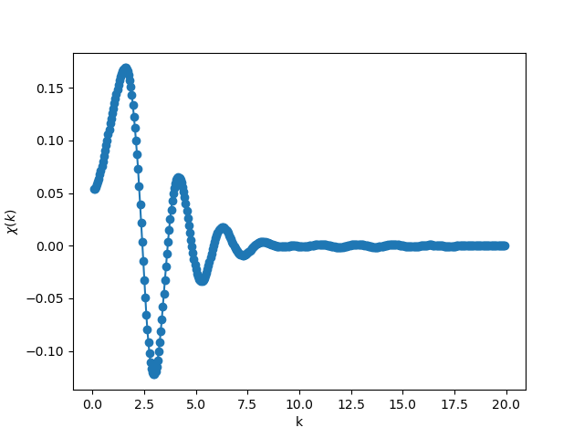
Fig. 1 An example of XAFS spectrum calculation using FEFF.