Optimization by Grid search
In this section, we will explain how to perform a grid-type search to analyze atomic coordinates from spectrum data. The grid type search is compatible with MPI. The search grid is generated from the input parameters as an evenly spaced mesh.
Location of the sample files
The sample files are located in sample/mapper.
The following files are stored in the folder:
mock_data.txt,template.txtReference file to proceed with calculations in the main program.
ref_ColorMap.txtA file to check if the calculation was performed correctly (the answer to
ColorMap.txtobtained by doing this tutorial).input.tomlInput file of the main program.
prepare.sh,do.shScript prepared for bulk calculation of this tutorial.
Below, we will describe these files and then show the actual calculation results.
Reference files
template.txt is a template of the input file for FEFF.
In this tutorial, to reduce the computational cost, we will perform the two-parameter search for the coordinates x, y of a sulfur atom, with z fixed to z = -1.60.
The content of the file is shown below in which @x and @y correspond to the parameters to be varied.
The reference data that imitates experiments is stored in the file mock_data.txt that contains the spectrum data for three different directions of polarization.
* This feff.inp file generated by ATOMS, version 2.50
* ATOMS written by and copyright (c) Bruce Ravel, 1992-1999

* -- * -- * -- * -- * -- * -- * -- * -- * -- * -- * -- * -- * -- * -- *
*       total mu =      725.4 cm^-1, delta mu =      610.0 cm^-1
*       specific gravity = 12.006, cluster contains   55 atoms.
* -- * -- * -- * -- * -- * -- * -- * -- * -- * -- * -- * -- * -- * -- *
*       mcmaster corrections:  0.00020 ang^2 and  0.770E-07 ang^4
* -- * -- * -- * -- * -- * -- * -- * -- * -- * -- * -- * -- * -- * -- *

TITLE   Sample_data

EDGE      K
S02       1.0

*         pot    xsph  fms   paths genfmt ff2chi
CONTROL   1      1      1      1      1      1
PRINT     0      0      0      0      0      0

*         r_scf   [ l_scf  n_scf  ca ]
*SCF       6.05142     0     15     0.1


EXAFS    20
RPATH    6

*         kmax  [ delta_k  delta_e ]
*XANES     4.0     0.07     0.5
*         r_fms     [ l_fms ]
*FMS       6.05142    0
*
*RPATH     0.10000
*         emin  emax  resolution
*LDOS      -20    20   0.1


POTENTIALS
*   ipot   z [ label   l_scmt  l_fms  stoichiometry ]
       0   28    Ni
       1   16    S
       2    8     O
NLEG         2

*CRITERIA     4.00     2.50

*DEBYE        300.00   340.00

* CORRECTION 4.50 0.5
* RMULTIPLIER 1.00
* ION 0 0.2
* ION 1 0.2

*         ixc  [ Vr  Vi ]
EXCHANGE  0    -5    0
SIG2  0.0016
POLARIZATION   @Ex @Ey @Ez

ATOMS
0.0000 0.0000 0.0000 0 Ni
@x @y -1.6000 1 S
1.1400 1.2800 0.9700 2 O
Input file
This section describes the input file for the main program, input.toml.
The details of input.toml can be found in the input file section of the manual.
The following is the content of input.toml in the sample file.
[base]
dimension = 2
output_dir = "output"

[solver]
name = "feff"

[solver.config]
feff_exec_file  = "feff85L"
feff_output_file = "chi.dat"
#remove_work_dir = true
#use_tmpdir = true

[solver.param]
string_list = ["@x", "@y"]
polarization_list = ["@Ex", "@Ey", "@Ez"]
polarization = [ [0,1,0], [1,0,0], [0,0,1] ]
calculated_first_k = 3.6
calculated_last_k = 10

[solver.reference]
path_epsilon = "mock_data.txt"

[algorithm]
name = "mapper"
label_list = ["x_S", "y_S"]

[algorithm.param]
min_list = [-2.0, -2.0]
max_list = [ 2.0,  2.0]
num_list = [21, 21]
First, [base] section is explained.
dimensionis the number of variables to be optimized. In this case, it is2since we are optimizing two variables as described intemplate.txt.output_diris the name of directory for the outputs. If it is omitted, the results are written in the directory in which the program is executed.
[solver] section specifies the solver to be used inside the main program and its settings.
nameis the name of the solver you want to use. In this tutorial it isfeff.
The solver can be configured in the subsections [solver.config], [solver.param], and [solver.reference].
[solver.config] section specifies options for feff85L called from the main program.
feff_exec_filespecifies the path to the FEFF executable.feff_output_filespecifies the file among the output files of FEFF that contains the XAFS spectrum data.remove_work_dirspecifies whether the work directory for the output of FEFF should be removed every after the calculation.use_tmpdirspecifies whether the output files of FEFF should be written in /tmp.
[solver.param] section specifies options for the input file of FEFF.
string_listis a list of variable names embedded intemplate.txt.polarization_listis a list of placeholders for the polarization vector embedded intemplate.txt.polarizationis a list of polarization vectors.calculated_first_k,calculated_last_kare the lower and upper ends of the wave number for which the calculated values and the experimental data are to be compared.
[solver.reference] section specifies the location of the experimental data and the range to read.
path_epsilonspecifies the path where the experimental data is located.
[algorithm] section specifies the algorithm to use and its settings.
nameis the name of the algorithm you want to use. In this tutorial we will usemappersince we will be using grid-search method.label_listis a list of label names to be attached to the output of@xand@y.
[algorithm.param] section specifies the options to the search algorithm.
min_list,max_list,num_listare the range of search grid and the number of grid points.
For details on other parameters that can be specified in the input file, please see the Input File section of the manual.
Calculation execution
First, move to the folder where the sample files are located. (We assume that you are directly under the directory where you downloaded this software.)
$ cd sample/mapper
Copy feff85L to the current directory.
$ cp ../feff/feff85L .
Run the main program. The computation time will take only a few minutes on a normal PC.
$ mpiexec -np 4 odatse-STR input.toml | tee log.txt
Here, the calculation using MPI parallel with 4 processes will be done.
When executed, a folder for each rank will be created, and a subfolder LogXXXX_YYYY (where XXXX and YYYY are the grid id and the sequence number, respectively) will be created under it.
The standard output will look like as follows.
name            : mapper
label_list      : ['x_S', 'y_S']
param.min_list  : [-2, -2]
param.max_list  : [2, 2]
param.num_list  : [21, 21]
Iteration : 1/441
@x = -2.00000000
@y = -2.00000000
R-factor = 19.739646449543752 Polarization [0.0, 1.0, 0.0] R-factor1 = 2.23082630928769  Polarization [1.0, 0.0, 0.0] R-factor2 = 3.745102742186708  Polarization [0.0, 0.0, 1.0] R-factor3 = 53.243010297156864
Iteration : 2/441
@x = -1.80000000
@y = -2.00000000
R-factor = 15.870615265918195 Polarization [0.0, 1.0, 0.0] R-factor1 = 2.465225144249503  Polarization [1.0, 0.0, 0.0] R-factor2 = 3.7116841611214517  Polarization [0.0, 0.0, 1.0] R-factor3 = 41.43493649238363
Iteration : 3/441
@x = -1.60000000
@y = -2.00000000
R-factor = 12.4966032440396 Polarization [0.0, 1.0, 0.0] R-factor1 = 3.4464214082242046  Polarization [1.0, 0.0, 0.0] R-factor2 = 2.6218600524063693  Polarization [0.0, 0.0, 1.0] R-factor3 = 31.421528271488228
Iteration : 4/441
@x = -1.40000000
@y = -2.00000000
R-factor = 11.698213396270965 Polarization [0.0, 1.0, 0.0] R-factor1 = 3.4791684719050933  Polarization [1.0, 0.0, 0.0] R-factor2 = 1.6240174174998872  Polarization [0.0, 0.0, 1.0] R-factor3 = 29.991454299407913
Iteration : 5/441
@x = -1.20000000
@y = -2.00000000
R-factor = 14.299726412681139 Polarization [0.0, 1.0, 0.0] R-factor1 = 2.2280314879817467  Polarization [1.0, 0.0, 0.0] R-factor2 = 1.5332463231108493  Polarization [0.0, 0.0, 1.0] R-factor3 = 39.13790142695082
Iteration : 6/441
@x = -1.00000000
@y = -2.00000000
R-factor = 21.44097816422594 Polarization [0.0, 1.0, 0.0] R-factor1 = 3.7563622860968673  Polarization [1.0, 0.0, 0.0] R-factor2 = 1.810765574876649  Polarization [0.0, 0.0, 1.0] R-factor3 = 58.7558066317043
Iteration : 7/441
@x = -0.80000000
@y = -2.00000000
R-factor = 28.455902096414444 Polarization [0.0, 1.0, 0.0] R-factor1 = 6.512305703044855  Polarization [1.0, 0.0, 0.0] R-factor2 = 2.004528093101423  Polarization [0.0, 0.0, 1.0] R-factor3 = 76.85087249309706
...
@x and @y are the candidate parameters for each mesh and R-factor is the function value at that point.
Finally, the R-factor calculated at all the points on the grid will be written to ColorMap.txt.
In this case, the following results will be obtained.
-2.000000 -2.000000 19.739646
-1.800000 -2.000000 15.870615
-1.600000 -2.000000 12.496603
-1.400000 -2.000000 11.698213
-1.200000 -2.000000 14.299726
-1.000000 -2.000000 21.440978
-0.800000 -2.000000 28.455902
...
The first and second columns contain the values of @x and @y, respectively, and the third column contains the R-factor.
Note that do.sh is available as a script for batch calculation.
In do.sh, res.txt and ref.txt are also compared for the check.
Here is what it does, without further explanation.
#!/bin/sh

sh prepare.sh

time mpiexec -np 4 odatse-XAFS input.toml

echo diff output/ColorMap.txt ref_ColorMap.txt
res=0
diff output/ColorMap.txt ref_ColorMap.txt || res=$?
if [ $res -eq 0 ]; then
  echo TEST PASS
  true
else
  echo TEST FAILED: ColorMap.txt and ref_ColorMap.txt differ
  false
fi
Visualization of calculation results
By examining ColorMap.txt, we can estimate the region where the value of R-factor becomes small.
In this case, the following command will create a plot on a two-dimensional plot of the parameter space in ColorMapFig.png.
$ python3 plot_colormap_2d.py -o ColorMapFig.png
Looking at the generated figure, we can see that it has the minimum value around (\(\pm 1.2\), \(\pm 0.8\)).
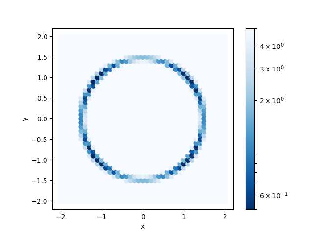
Fig. 2 Color map of R-factor with respect to x and y coordinates of S atom at z=-1.60.