Optimization by replica exchange Monte Carlo method
This tutorial describes how to estimate atomic positions from the experimental diffraction data by using the replica exchange Monte Carlo method (RXMC).
Sample files
Sample files are available from sample/single_beam/exchange .
This directory includes the following files:
bulk.txtThe input file of
bulk.exe.experiment.txt,template.txtReference files for the main program.
ref.txtSolution file for checking whether the calucation is successful or not.
input.tomlThe input file of the main program.
prepare.sh,do.shScript files for running this tutorial.
In the following, we will describe these files and then show the result.
Reference files
This tutorial uses the reference files, template.txt and experiment.txt,
which are the same as those used in the previous tutorial (Optimization by Nelder-Mead method).
Input files
This subsection describes the input files.
For details, see the replica exchange Monte Carlo method in ODAT-SE manual.
input.toml in the sample directory is shown as the following:
[base]
dimension = 2
output_dir = "output"

[algorithm]
name = "exchange"
label_list = ["z1", "z2"]
seed = 12345

[algorithm.param]
min_list = [3.0, 3.0]
max_list = [6.0, 6.0]
step_list = [1.0, 1.0]

[algorithm.exchange]
numsteps = 1000
numsteps_exchange = 20
Tmin = 0.005
Tmax = 0.05
Tlogspace = true

[solver]
name = "sim-trhepd-rheed"
run_scheme = "subprocess"

[solver.config]
cal_number = [1]

[solver.param]
string_list = ["value_01", "value_02" ]
degree_max = 7.0

[solver.reference]
path = "experiment.txt"
exp_list = [1]

[solver.post]
normalization = "TOTAL"
In the following, we will briefly describe the contents of the file. For details, see the algorithm section of ODAT-SE manual.
[base] section describes the settings for a whole calculation.
dimensionis the number of variables you want to optimize. In this case, specify2because it optimizes two variables.output_diris the name of directory for the outputs. If it is omitted, the results are written in the directory in which the program is executed.
[solver] section specifies the solver to use inside the main program and its settings.
See the minsearch tutorial.
[algorithm] section sets the algorithm to use and its settings.
nameis the name of the algorithm you want to use. In this tutorial we will use RXMC, so specifyexchange.label_listis a list of labels to be attached to the output ofvalue_0x(x = 1,2).seedis the seed that a pseudo-random number generator uses.
[algorithm.param] section sets the parameter space to be explored.
min_listis a lower bound andmax_listis an upper bound.step_listspecifies the step size of one Monte Carlo update (deviation of Gaussian).
[algorithm.exchange] section sets the parameters for RXMC.
numstepis the number of Monte Carlo steps.numsteps_exchangeis the number of interval steps between temperature exchanges.Tmin,Tmaxare the minimum and the maximum of temperature, respectively.When
Tlogspaceistrue, the temperature points are distributed uniformly in the logarithmic space.
[solver] section specifies the solver to use inside the main program and its settings.
See the Optimization by Nelder-Mead method tutorial.
Calculation
First, move to the folder where the sample file is located. (Hereinafter, it is assumed that you are the root directory of odatse-STR.)
$ cd sample/single_beam/exchange
Copy bulk.exe and surf.exe as in the tutorial for the direct problem.
$ cp ../../sim-trhepd-rheed/src/bulk.exe .
$ cp ../../sim-trhepd-rheed/src/surf.exe .
Execute bulk.exe to generate bulkP.b .
$ ./bulk.exe
Then, run the main program. It will take a few secondes on a normal PC.
$ mpiexec -np 4 odatse-STR input.toml | tee log.txt
Here, the calculation is performed using MPI parallel with 4 processes.
If you are using Open MPI and you request more processes than the number of available CPU cores, add the --oversubscribed option to the mpiexec command.
When executed, a folder for each rank will be created under the directory output, and trial.txt and result.txt will be created.
trial.txt contains the parameters evaluated in each Monte Carlo step and the value of the objective function, and result.txt contains the parameters actually adopted.
These files have the same format: the first two columns are time (step) and the index of walker in the process, the third is the temperature, the fourth column is the value of the objective function, and the fifth and subsequent columns are the parameters.
# step walker T fx x1 x2
0 0 0.004999999999999999 0.07830821484593968 3.682008067401509 3.9502750191292586
1 0 0.004999999999999999 0.07830821484593968 3.682008067401509 3.9502750191292586
2 0 0.004999999999999999 0.07830821484593968 3.682008067401509 3.9502750191292586
3 0 0.004999999999999999 0.06273922648753057 4.330900869594549 4.311333132184154
In the case of the sim-trhepd-rheed solver, a subfolder LogXXXX_YYYY (XXXX is the number of MC steps) is created under each working directory, and the rocking curve information and other outputs are recorded.
result.txt in the output directory for each MPI rank records the data sampled by each replica. They are rearranged according to the temperature, and stored in the files output/result_T*.txt in which * stands for the index of the temperature.
Finally, best_result.txt is filled with the information about the parameters with the value of the optimal objective function (R-factor), the rank from which it was obtained, and the Monte Carlo step.
nprocs = 4
rank = 1
step = 282
walker = 0
fx = 0.008414800224430936
z1 = 5.164773671165013
z2 = 4.226467514644945
In addition, do.sh is prepared as a script for batch calculation.
do.sh also checks the difference between best_result.txt and ref.txt.
The content of the script is shown below, though further information will be omitted.
#!/bin/sh

sh prepare.sh

./bulk.exe

time mpiexec --oversubscribe -np 4 odatse-STR input.toml

echo diff output/best_result.txt ref.txt
res=0
diff best_result.txt ref.txt || res=$?
if [ $res -eq 0 ]; then
  echo TEST PASS
  true
else
  echo TEST FAILED: best_result.txt and ref.txt differ
  false
fi
Visualization
By illustrating output/result_T*.txt, you can estimate regions where the parameters with small R-factor are.
In this case, the figure result.png of the 2D parameter space is created for the data in output/result_T1.txt by using the following command.
$ python3 plot_result_2d.py
Looking at the resulting diagram, we can see that the samples are concentrated near (5.25, 4.25) and (4.25, 5.25), and that the R-factor value is small there.
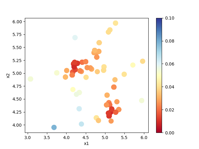
Fig. 5 Sampled parameters and R-factor. The horizontal axes is x1 (value_01) and the vertical axes is x2 (value_02).
Also, RockingCurve.txt is stored in each subfolder
LogXXXX_YYYY (XXXX is the index of MC step and YYYY is the index of replica in the MPI process) when generate_rocking_curve in [solver] section is set to true.
By using this, it is possible to compare the result with the experimental value according to the procedure of the previous tutorial.